A system cannot be successful if it is too strongly influenced by a single person. Once the initial design is complete and fairly robust, the real test begins as people with many different viewpoints undertake their own experiments. —Donald Knuth
- Three different types of systems:
- Services (online systems): Response time is usually the primary measure of performance of a service and availability is often very important. (e.g. API)
- Batch processing systems (offline systems): primary performance measure of a batch job is usually throughput (the time it takes to crunch through an input dataset of a certain size). (e.g. MapReduce)
- Stream processing systems (near-real-time systems): As stream processing builds upon batch processing. (e.g. Kafka)
- As we shall see in this chapter, batch processing is an important building block in our quest to build reliable, scalable, and maintainable applications. (e.g. MapReduce → Hadoop, CouchDB, and MongoDB)
Batch Processing with Unix Tools
- Simple Log Analysis
- Surprisingly many data analyses can be done in a few minutes using some combination of awk, sed, grep, sort, uniq, and xargs, and they perform surprisingly well.
- Chain of commands vs. Custom program:
- Instead of the chain of Unix commands, you could write a simple program to do the same thing. (e.g. Ruby, Python)
- Sorting vs. in-memory aggregation:
- The sort utility in GNU Coreutils (Linux) automatically handles larger-than-memory datasets by spilling to disk, and automatically parallelized sorting across multiple CPU cores.
- This means that the simple chain of Unix commands we saw earlier easily scales to large datasets, without running out of memory. (Limited by desk speed)
- The sort utility in GNU Coreutils (Linux) automatically handles larger-than-memory datasets by spilling to disk, and automatically parallelized sorting across multiple CPU cores.
- The Unix Philosophy
- Doug McIlroy from 1964 “We should have some ways of connecting programs like [a] garden hose—screw in another segment when it becomes necessary to massage data in another way. This is the way of I/O also.”
- The idea of connecting programs with pipes became part of what is now known as the Unix philosophy—a set of design principles that became popular among the developers and users of Unix.
- This approach—automation, rapid prototyping, incremental iteration, being friendly to experimentation, and breaking down large projects into manageable chunks— sounds remarkably like the Agile and DevOps movements of today.
- A uniform interface:
- In Unix, that interface is a file (or, more precisely, a file descriptor).
- Another example of a uniform interface is URLs and HTTP, the foundations of the web.
- A file is just an ordered sequence of bytes.
- In Unix, that interface is a file (or, more precisely, a file descriptor).
- Separation of logic and wiring:
- Another characteristic feature of Unix tools is their use of standard input (stdin) and standard output (stdout).
- Separating the input/output wiring from the program logic makes it easier to compose small tools into bigger systems.
- Transparency and experimentation:
- Part of what makes Unix tools so successful is that they make it quite easy to see what is going on.
- the biggest limitation of Unix tools is that they run only on a single machine—and that’s where tools like Hadoop come in.
MapReduce and Distributed Filesystems
- MapReduce is a bit like Unix tools, but distributed across potentially thousands of machines.
- Like Unix tools, it is a fairly blunt, brute-force, but surprisingly effective tool.
- A single MapReduce job is comparable to a single Unix process: it takes one or more inputs and produces one or more outputs.
- Instead of stdin or stdout, MapReduce jobs read and write files on a distributed filesystem. (e.d. HDFS for Hadoop, open source version of GFS)
- GlusterFS and the Quantcast File System (QFS). Object storage services such as Amazon S3, Azure Blob Storage, and OpenStack Swift are similar in many ways.
- HDFS is based on the shared-nothing principle (see the introduction to Part II), in contrast to the shared-disk approach of Network Attached Storage (NAS) and Storage Area Network (SAN) architectures.
- shared-nothing approach requires no special hardware, only computers connected by a conventional data center network.
- HDFS consists of a daemon process running on each machine, exposing a network service that allows other nodes to access files stored on that machine (assuming that every general-purpose machine in a datacenter has some disks attached to it).
- A central server called the NameNode keeps track of which file blocks are stored on which machine.
- Thus, HDFS conceptually creates one big filesystem that can use the space on the disks of all machines running the daemon.
- In order to tolerate machine and disk failures, file blocks are replicated on multiple machines.
- ensure coding scheme such as Reed–Solomon codes, kind like RAID.
- HDFS has scaled well: at the time of writing, the biggest HDFS deployments run on tens of thousands of machines, with combined storage capacity of hundreds of petabytes.
- MapReduce Job Execution:
- MapReduce is a programming framework with which you can write code to process large datasets in a distributed filesystem like HDFS.
- To create a MapReduce job, you need to implement two callback functions:
- Mapper: The mapper is called once for every input record, and its job is to extract the key and value from the input record.
- Reducer: The MapReduce framework takes the key-value pairs produced by the mappers, collects all the values belonging to the same key, and calls the reducer with an iterator over that collection of values.
- Viewed like this;
- The role of the mapper is to prepare the data by putting it into a form that is suitable for sorting.
- The role of the reducer is to process the data that has been sorted.
- Distributed execution of MapReduce:
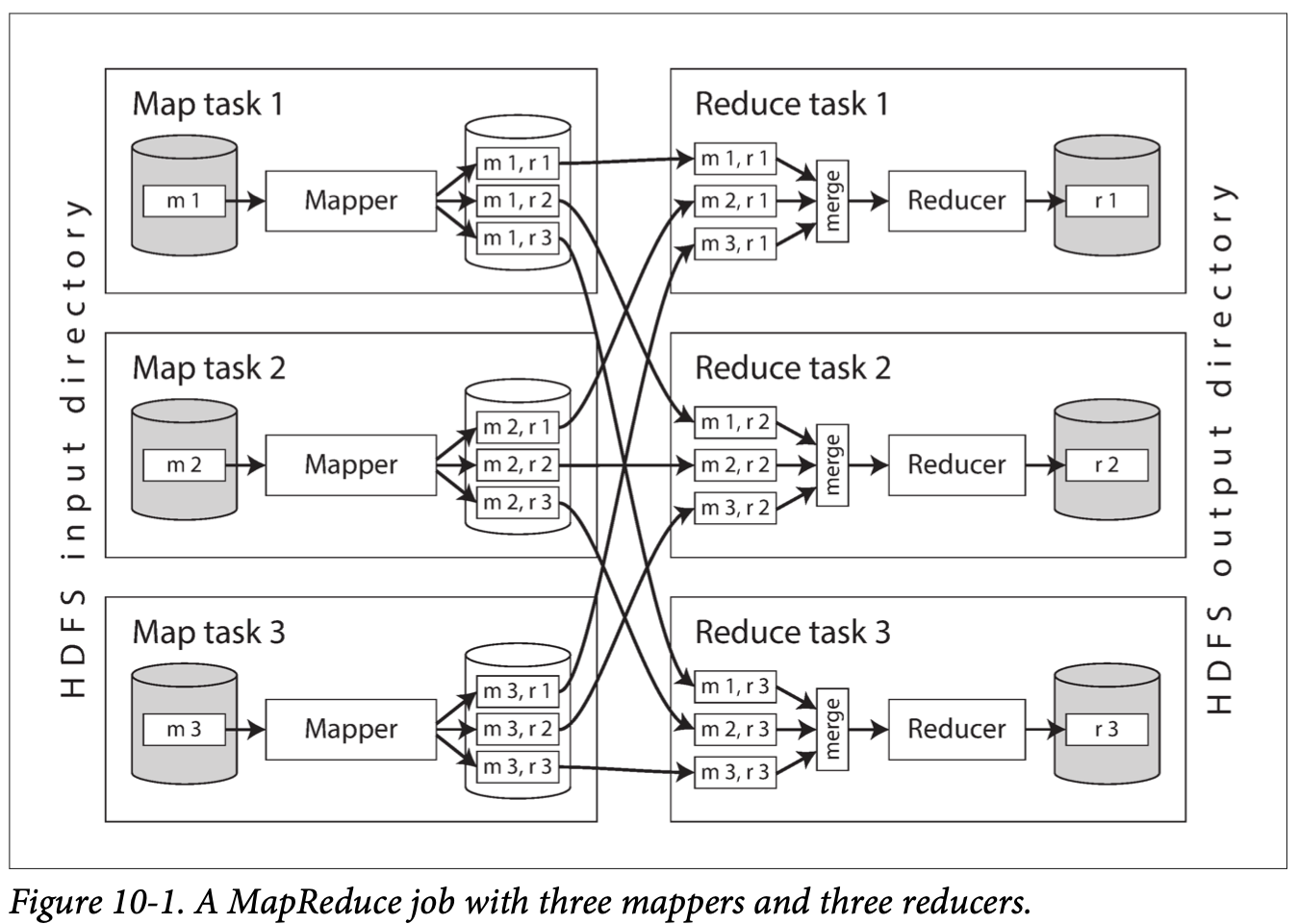
- parallelization is based on partitioning
- Putting the computation near the data: it saves copying the input file over the network, reducing network load and increasing locality.
- The reduce side of the computation is also partitioned.
- The key-value pairs must be sorted, but the dataset is likely too large to be sorted with a conventional sorting algorithm on a single machine. Instead, the sorting is performed in stages.
- The process of partitioning by reducer, sorting, and copying data partitions from mappers to reducers is known as the shuffle.
- MapReduce workflows:
- it is very common for MapReduce jobs to be chained together into workflows, such that the output of one job becomes the input to the next job.
- this chaining is done implicitly by directory name:
- First job must be configured to write its output to a designated directory in HDFS,
- Second job must be configured to read that same directory name as its input.
- Various workflow schedulers for Hadoop have been developed, including Oozie, Azkaban, Luigi, Airflow, and Pinball
- Workflows consisting of 50 to 100 MapReduce jobs are common when building recommendation systems.
- Various higher-level tools for Hadoop, such as Pig, Hive, Cascading, Crunch, and FlumeJava.
- it is very common for MapReduce jobs to be chained together into workflows, such that the output of one job becomes the input to the next job.
- Reduce-Side Joins and Grouping:
- A foreign key in a relational model, a document reference in a document model, or an edge in a graph model.
- MapReduce has no concept of indexes—at least not in the usual sense.
- Example: analysis of user activity events:
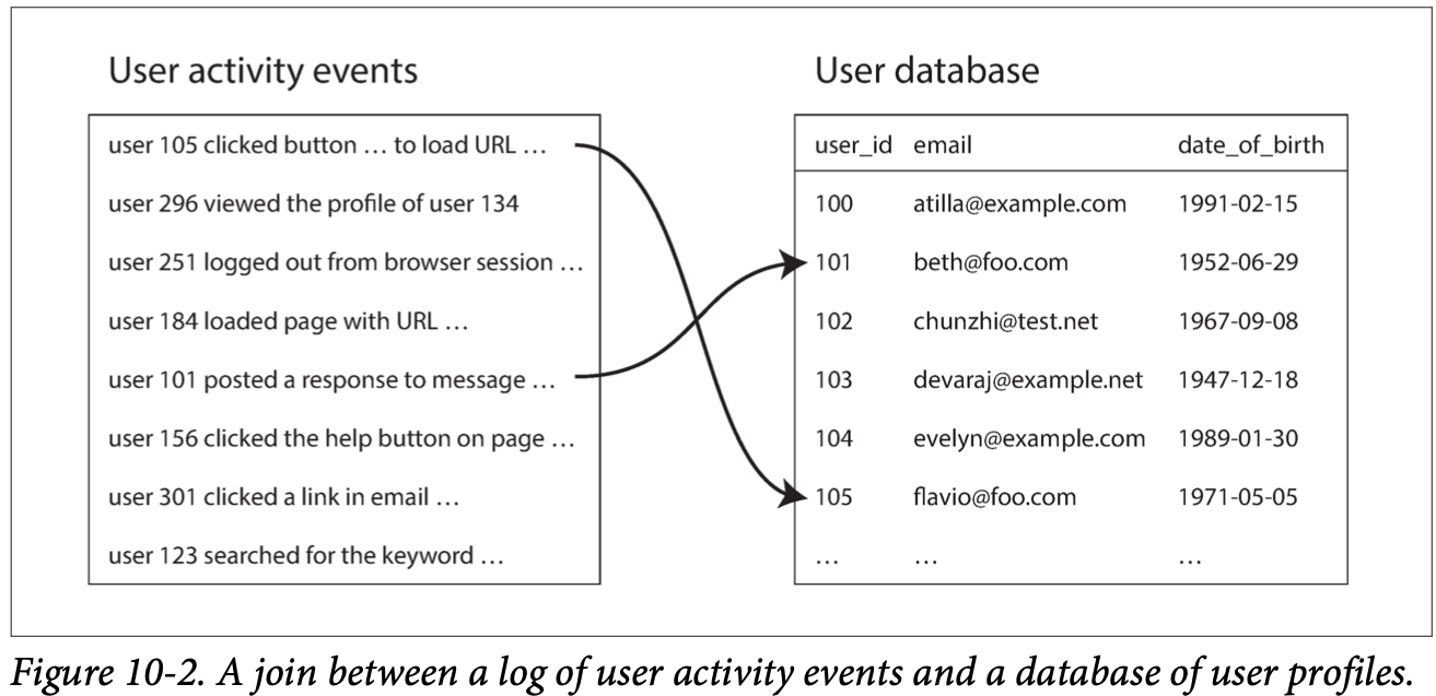
- Star schema: the log of events is the fact table, and the user database is one of the dimensions.
- In order to achieve good throughput in a batch process, the computation must be (as much as possible) local to one machine.
- Sort-merge joins:
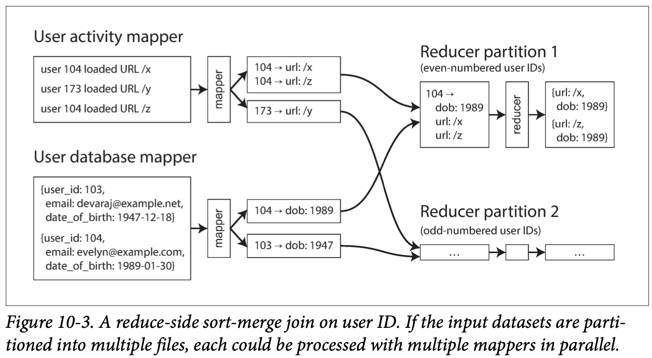
- The effect is that all the activity events and the user record with the same user ID become adjacent to each other in the reducer input. (along with secondary sort)
- sort-merge join: Since the reducer processes all of the records for a particular user ID in one go, it only needs to keep one user record in memory at any one time, and it never needs to make any requests over the network. (C: this explained why ETL tool Pentaho/Kettle need to always sort the value before “Merge Join Row”)
- Bringing related data together in the same place:
- One way of looking at this architecture is that mappers “send messages” to the reducers.
- When a mapper emits a key-value pair, the key acts like the destination address to which the value should be delivered.
- Using the MapReduce programming model has separated the physical network communication aspects of the computation (getting the data to the right machine) from the application logic (processing the data once you have it).
- One way of looking at this architecture is that mappers “send messages” to the reducers.
- GROUP BY:
- The simplest way is to set up the mappers so that the key-value pairs they produce use the desired grouping key.
- Another common use for grouping is collating all the activity events for a particular user session, in order to find out the sequence of actions that the user took—a process called sessionization. (e.g. for A/B testing)
- Handling skew:
- The pattern of “bringing all records with the same key to the same place” breaks down if there is a very large amount of data related to a single key.
- e.g. celebrities in SNS, Such disproportionately active database records are known as linchpin objects or hot keys.
- If a join input has hot keys, there are a few algorithms you can use to compensate. (e.g. skewed join method in Pig, sharded join method in Crunch)
- Hive’s skewed join optimization takes an alternative approach.
- When grouping records by a hot key and aggregating them, you can perform the grouping in two stages.
- The pattern of “bringing all records with the same key to the same place” breaks down if there is a very large amount of data related to a single key.
- Map-Side Joins:
- The reduce-side approach has the advantage that you do not need to make any assumptions about the input data.
- if you can make certain assumptions about your input data, it is possible to make joins faster by using a so-called map-side join.
- This approach uses a cut-down MapReduce job in which there are no reducers and no sorting.
- Broadcast hash joins:
- The simplest way of performing a map-side join applies in the case where a large dataset is joined with a small dataset.
- the small dataset needs to be small enough that it can be loaded entirely into memory in each of the mappers
- This simple but effective algorithm is called a broadcast hash join:
- The word broadcast reflects the fact that each mapper for a partition of the large input reads the entirety of the small input (so the small input is effectively “broadcast” to all partitions of the large input), and the word hash reflects its use of a hash table.
- E.g. Pig (under the name “replicated join”), Hive (“MapJoin”), Cascading, and Crunch, Data-warehouse engine Impala.
- Instead of loading the small join input into an in-memory hash table, an alternative is to store the small join input in a read-only index on the local disk. (fit in OS’ page cache, almost as fast as memory)
- The simplest way of performing a map-side join applies in the case where a large dataset is joined with a small dataset.
- Partitioned hash joins: (e.g. bucketed map joins in Hive)
- If the inputs to the map-side join are partitioned in the same way, then the hash join approach can be applied to each partition independently.
- This approach only works if both of the join’s inputs have the same number of partitions, with records assigned to partitions based on the same key and the same hash function.
- Map-side merge joins:
- not only partitioned in the same way, but also sorted based on the same key.
- MapReduce workflows with map-side joins:
- When the output of a MapReduce join is consumed by downstream jobs, the choice of map-side or reduce-side join affects the structure of the output.
- Knowing about the physical layout of datasets in the distributed filesystem becomes important when optimizing join strategies.
- In the Hadoop ecosystem, this kind of metadata about the partitioning of datasets is often maintained in HCatalog and the Hive metastore.
- The Output of Batch Workflows:
- Where does batch processing fit in?
- It is not transaction processing, nor is it analytics. It is closer to analytics, in that a batch process typically scans over large portions of an input dataset.
- The output of a batch process is often not a report, but some other kind of structure.
- Building search indexes: (documents in, indexes out.)
- Google’s original use of MapReduce was to build indexes for its search engine, which was implemented as a workflow of 5 to 10 MapReduce jobs. (e.g. still used today by Lucene/Solr)
- Recall full-text search index: it is a file (the term dictionary) in which you can efficiently look up a particular keyword and find the list of all the document IDs containing that keyword (the postings list).
- Key-value stores as batch process output: (database files in, database out)
- Another common use for batch processing is to build machine learning systems such as classifiers (e.g., spam filters, anomaly detection, image recognition) and recommendation systems (e.g., people you may know, products you may be interested in, or related searches)
- Build a brand-new database inside the batch job and write it as files to the job’s output directory in the distributed filesystem, just like the search indexes in the last section.
- Various key-value stores support building database files in MapReduce jobs, including Voldemort, Terrapin, ElephantDB, and HBase bulk loading.
- Philosophy of batch process outputs:
- In the process, the input is left unchanged, any previous output is completely replaced with the new output, and there are no other side effects.
- By treating inputs as immutable and avoiding side effects (such as writing to external databases), batch jobs not only achieve good performance but also become much easier to maintain.
- On Hadoop, some of those low-value syntactic conversions are eliminated by using more structured file formats: e.g. Avro, Parquet
- Where does batch processing fit in?
- Comparing Hadoop to Distributed Databases:
- Hadoop is somewhat like a distributed version of Unix, where HDFS is the filesystem and MapReduce is a quirky implementation of a Unix process(which happens to always run the sort utility between the map phase and the reduce phase).
- MapReduce and a Distributed Filesystem provides something much more like a general-purpose operating system that can run arbitrary programs.
- Diversity of storage:
- Databases require you to structure data according to a particular model (e.g., relational or documents),
- whereas files in a distributed filesystem are just byte sequences, which can be written using any data model and encoding.
- Collecting data in its raw form, and worrying about schema design later, allows the data collection to be speeded up (a concept sometimes known as a “data lake” or “enterprise data hub” ).
- Aka. sushi principle: “raw (data) is better”
- Indiscriminate data dumping shifts the burden of interpreting the data from producer to consumer’s problem (schema-on-read approach).
- There may not even be one ideal data model, but rather different views onto the data that are suitable for different purposes.
- Data modeling still happens, but it is in a separate step, decoupled from the data collection.
- This decoupling is possible because a distributed filesystem supports data encoded in any format.
- Databases require you to structure data according to a particular model (e.g., relational or documents),
- Diversity of processing models:
- MapReduce gave engineers the ability to easily run their own code over large datasets.
- Sometimes having two processing models, SQL and MapReduce, was not enough.
- The system is flexible enough to support a diverse set of workloads within the same cluster.
- Not having to move data around makes it a lot easier to derive value from the data, and a lot easier to experiment with new processing models.
- Designing for frequent faults:
- When comparing MapReduce to MPP databases, two more differences in design approach stand out: the handling of faults and the use of memory and disk.
- MPP databases prefer to keep as much data as possible in memory (e.g., using hash joins) to avoid the cost of reading from disk.
- MapReduce is very eager to write data to disk, partly for fault tolerance, and partly on the assumption that the dataset will be too big to fit in memory anyway.
- Overcommitting resources in turn allows better utilization of machines and greater efficiency compared to systems that segregate production and non-production tasks.
- It’s not because the hardware is particularly unreliable, it’s because the freedom to arbitrarily terminate processes enables better resource utilization in a computing cluster.
- Among open source cluster schedulers, preemption is less widely used. (e.g. YARN’s CapacityScheduler)
- When comparing MapReduce to MPP databases, two more differences in design approach stand out: the handling of faults and the use of memory and disk.
Beyond MapReduce
- Depending on the volume of data, the structure of the data, and the type of processing being done with it, other tools may be more appropriate for expressing a computation.
- Implementing a complex processing job using the raw MapReduce APIs is actually quite hard and laborious—for instance, you would need to implement any join algorithms from scratch.
- In response to the difficulty of using MapReduce directly, various higher-level programming models (Pig, Hive, Cascading, Crunch) were created as abstractions on top of MapReduce.
- Materialization of Intermediate State:
- Publishing data to a well-known location in the distributed file system allows loose coupling so that jobs don’t need to know who is producing their input or consuming their output.
- Intermediate state: a means of passing data from one job to the next. (not shared between job or team)
- The process of writing out this intermediate state to files is called materialization. (C: recall “materialized views” from previously)
- In contrast: Pipes do not fully materialize the intermediate state, but instead stream the output to the input incrementally, using only a small in-memory buffer.
- MapReduce’s approach of fully materializing intermediate state has downsides compared to Unix pipes: (C: which derived from its advantages)
- A MapReduce job can only start when all tasks in the preceding jobs (that generate its inputs) have completed;
- Mappers are often redundant: they just read back the same file that was just written by a reducer, and prepare it for the next stage of partitioning and sorting.
- Storing intermediate state in a distributed file system means those files are replicated across several nodes, which is often overkill for such temporary data.
- Dataflow engines:
- New execution engine created to solve previou problems. E.g. Spark, Tez, and Flink.
- They handle an entire workflow as one job, rather than breaking it up into independent subjobs.
- Since they explicitly model the flow of data through several processing stages, these systems are known as dataflow engines.
- Offers several advantages compared to the MapReduce model:
- Expensive work such as sorting need only be performed in places where it is actually required.
- There are no unnecessary map tasks
- Can make locality optimizations.
- It is usually sufficient for intermediate state between operators to be kept in memory or written to local disk.
- Operators can start executing as soon as their input is ready;
- Existing Java Virtual Machine (JVM) processes can be reused to run new operators, reducing startup overheads compared to MapReduce (which launches a new JVM for each task).
- New execution engine created to solve previou problems. E.g. Spark, Tez, and Flink.
- Fault tolerance:
- An advantage of fully materializing intermediate state to a distributed file system is that it is durable, which makes fault tolerance fairly easy.
- if a task fails, it can just be restarted on another machine and read the same input again from the filesystem.
- Spark, Flink, and Tez avoid writing intermediate state to HDFS, so they take a different approach to tolerating faults:
- if a machine fails and the intermediate state on that machine is lost, it is recomputed from other data that is still available.
- To enable this recomputation, the framework must keep track of how a given piece of data was computed—which input partitions it used, and which operators were applied to it.
- When recomputing data, it is important to know whether the computation is deterministic.
- The solution in the case of non-deterministic operators is normally to kill the downstream operators as well, and run them again on the new data.
- In order to avoid such cascading faults, it is better to make operators deterministic.
- When recomputing data, it is important to know whether the computation is deterministic.
- Recovering from faults by recomputing data is not always the right answer:
- if the intermediate data is much smaller than the source data, or if the computation is very CPU-intensive, it is probably cheaper to materialize the intermediate data to files than to recompute it.
- An advantage of fully materializing intermediate state to a distributed file system is that it is durable, which makes fault tolerance fairly easy.
- Discussion of materialization:
- Flink especially is built around the idea of pipelined execution: that is, incrementally passing the output of an operator to other operators, and not waiting for the input to be complete before starting to process it.
- Graphs and Iterative Processing:
- In graph processing, the data itself has the form of a graph.
- This need often arises in machine learning applications such as recommendation engines, or in ranking systems. (e.g. PageRank)
- Iterative style: (works, but very inefficient with MapReduce)
- 1. An external scheduler runs a batch process to calculate one step of the algorithm.
- 2. When the batch process completes, the scheduler checks whether it has finished.
- 3. If it has not yet finished, the scheduler goes back to step 1 and runs another round of the batch process.
- The Pregel processing model:
- As an optimization for batch processing graphs, the bulk synchronous parallel (BSP) model of computation has become popular. Aka. “Pregel model”.
- (implemented by Apache Giraph, Spark’s GraphX API, and Flink’s Gelly API.)
- Idea behind Pregel: one vertex can “send a message” to another vertex, and typically those messages are sent along the edges in a graph.
- In each iteration, a function is called for each vertex, passing it all the messages that were sent to it—much like a call to the reducer. (It’s a bit similar to the actor model)
- As an optimization for batch processing graphs, the bulk synchronous parallel (BSP) model of computation has become popular. Aka. “Pregel model”.
- Fault tolerance:
- Pregel implementations guarantee that messages are processed exactly once at their destination vertex in the following iteration.
- This fault tolerance is achieved by periodically check-pointing the state of all vertices at the end of an iteration. (i.e., writing their full state to durable storage.)
- Parallel execution:
- A vertex does not need to know on which physical machine it is executing; when it sends messages to other vertices, it simply sends them to a vertex ID.
- High-Level APIs and Languages:
- Spark and Flink also include their own high-level dataflow APIs, often taking inspiration from FlumeJava.
- These dataflow APIs generally use relational-style building blocks to express a computation:
- joining datasets on the value of some field;
- grouping tuples by key;
- filtering by some condition;
- and aggregating tuples by counting, summing, or other functions.
- The move toward declarative query languages:
- The choice of join algorithm can make a big difference to the performance of a batch job;
- This is possible if joins are specified in a declarative way: the application simply states which joins are required, and the query optimizer decides how they can best be executed.
- Hive, Spark DataFrames, and Impala also use vectorized execution: iterating over data in a tight inner loop that is friendly to CPU caches, and avoiding function calls.
- batch processing frameworks begin to look more like MPP databases (and can achieve comparable performance) they retain their flexibility advantage.
- Specialization for different domains:
- Another domain of increasing importance is statistical and numerical algorithms, which are needed for machine learning applications such as classification and recommendation systems.
Summary
- In this chapter we explored the topic of batch processing.
- In the Unix world, the uniform interface that allows one program to be composed with another in files and pipes;
- In MapReduce, that interface is a distributed file system.
- Dataflow engines add their own pipe-like data transport mechanisms to avoid materializing intermediate state to the distributed file system, but the initial input and final output of a job is still usually HDFS.
- The two main problems that distributed batch processing frameworks need to solve are:
- Partitioning: In MapReduce, mappers are partitioned according to input file blocks.
- Fault tolerance: MapReduce frequently writes to disk, which makes it easy to recover from an individual failed task.
- Join algorithms for MapReduce:
- Sort-merge joins: Each of the inputs being joined goes through a mapper that extracts the join key.
- Broadcast hash joins: One of the two join inputs is small, so it is not partitioned and it can be entirely loaded into a hash table.
- Partitioned hash joins: If the two join inputs are partitioned in the same way (using the same key, same hash function, and same number of partitions), then the hash table approach can be used independently for each partition.
- Distributed batch processing engines have a deliberately restricted programming model: callback functions (such as mappers and reducers) are assumed to be stateless and to have no externally visible side effects besides their designated output.
- Does not need to worry about implementing fault-tolerance mechanisms: the framework can guarantee that the final output of a job is the same as if no faults had occurred, even though in reality various tasks perhaps had to be retried.
- The output is derived from the input. And the input data is bounded: it has a known, fixed size (for example, it consists of a set of log files at some point in time, or a snapshot of a database’s contents).